UPDATE: more efficient solutions have been proposed, uniform_filter1d from scipy being probably the best among the “standard” 3rd-party libraries, and some newer or specialized libraries are available too.
You can use np.convolve for that:
np.convolve(x, np.ones(N)/N, mode='valid')
Explanation
The running mean is a case of the mathematical operation of convolution. For the running mean, you slide a window along the input and compute the mean of the window’s contents. For discrete 1D signals, convolution is the same thing, except instead of the mean you compute an arbitrary linear combination, i.e., multiply each element by a corresponding coefficient and add up the results. Those coefficients, one for each position in the window, are sometimes called the convolution kernel. The arithmetic mean of N values is (x_1 + x_2 + ... + x_N) / N, so the corresponding kernel is (1/N, 1/N, ..., 1/N), and that’s exactly what we get by using np.ones(N)/N.
Edges
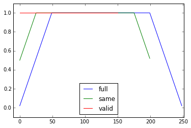
The mode argument of np.convolve specifies how to handle the edges. I chose the valid mode here because I think that’s how most people expect the running mean to work, but you may have other priorities. Here is a plot that illustrates the difference between the modes:
import numpy as np
import matplotlib.pyplot as plt
modes = ['full', 'same', 'valid']
for m in modes:
    plt.plot(np.convolve(np.ones(200), np.ones(50)/50, mode=m));
plt.axis([-10, 251, -.1, 1.1]);
plt.legend(modes, loc='lower center');
plt.show()