You need to specify the arguments to forecast() a little differently; since you didn’t post example data, I’ll demonstrate with the gold dataset in the forecast package:
library(forecast)
data(gold)
trainingData <- gold[1:554]
testData <- gold[555:1108]
fitModel <- Arima(trainingData, order=c(2, 0, 3))
ForcastData <- forecast(fitModel, testData)
# Error in rep(1, n.ahead) : invalid 'times' argument
ForcastData <- forecast(object=testData, model=fitModel) # no error
accuracy(f=ForcastData) # you only need to give ForcastData; see help(accuracy)
                    ME     RMSE      MAE        MPE      MAPE     MASE
Training set 0.4751156 6.951257 3.286692 0.09488746 0.7316996 1.000819
                   ACF1
Training set -0.2386402
You may want to spend some time with the forecast package documentation to see what the arguments for the various functions are named and in what order they appear.
Regarding your forecast.Arima not found error, you can see this answer to a different question regarding the forecast package — essentially that function isn’t meant to be called by the user, but rather called by the forecast function.
EDIT:
After receiving your comment, it seems the following might help:
library(forecast)
# Read in the data
full_data <- read.csv('~/Downloads/onevalue1.csv')
full_data$UnixHour <- as.Date(full_data$UnixHour)
# Split the sample
training_indices <- 1:floor(0.7 * nrow(full_data))
training_data <- full_data$Lane1Flow[training_indices]
test_data <- full_data$Lane1Flow[-training_indices]
# Use automatic model selection:
autoARIMAFastTrain1 <- auto.arima(training_data, trace=TRUE, ic ="aicc",
approximation=FALSE, stepwise=FALSE)
# Fit the model on test data:
fit_model <- Arima(training_data, order=c(2, 0, 3))
# Do forecasting
forecast_data <- forecast(object=test_data, model=fit_model)
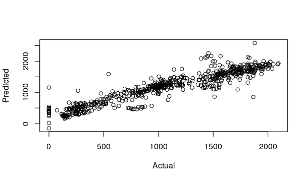
# And plot the forecasted values vs. the actual test data:
plot(x=test_data, y=forecast_data$fitted, xlab='Actual', ylab='Predicted')
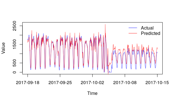
# It could help more to look at the following plot:
plot(test_data, type='l', col=rgb(0, 0, 1, alpha=0.7),
     xlab='Time', ylab='Value', xaxt='n', ylim=c(0, max(forecast_data$fitted)))
ticks <- seq(from=1, to=length(test_data), by=floor(length(test_data)/4))
times <- full_data$UnixHour[-training_indices]
axis(1, lwd=0, lwd.ticks=1, at=ticks, labels=times[ticks])
lines(forecast_data$fitted, col=rgb(1, 0, 0, alpha=0.7))
legend('topright', legend=c('Actual', 'Predicted'), col=c('blue', 'red'),
       lty=1, bty='n')